Table of Contents
Introduction
Consider the following mathematical representation of a pendulum

Dynamics
Solutions
There does not exist a closed form solution for all initial conditions for all time of the pendulum in terms of elementary functions 1. This however does not mean that we cannot characterize certain aspects of the system, which we will do in subsequent sections. By numerically integrating, we can construct a sample phase portrait (positions versus velocities) for a pendulum with damping:

Euler-Lagrange
The Euler-Lagrange method is an energy-based method for constructing the equations of motion of the system. To begin, we note that the rotational kinetic energy of the system $T:\mathcal{X}\to \mathbb{R}$ is given by $T(x)=\frac{1}{2}ml^2\dot{\theta}^2$, and the potential energy of the system $V:\mathcal{Q}\to\mathbb{R}$ by $V=mgl(1-\cos\theta)$. We can therefore construct the Lagrangian as
\begin{align}
L&=T-V\notag \\ \notag
&=\frac{1}{2}ml^2\dot{\theta}^2-mgl(1-\cos\theta).\notag
\end{align}
We can represent the damping force as a Rayleigh dissipation function with $\mathcal{F}=\frac{1}{2}b\dot{\theta}^2$. This gives us a force in the generalized coordinates of
\[
Q_i = -\frac{\partial\mathcal{F}}{\partial\dot{\theta}}=-b\dot{\theta}.
\]
Employing the Lagrange d’Alembert principle results in the equations of motion of the system, as given by
\begin{align}
\frac{d}{dt}\left(\frac{\partial L}{\partial v^i}\right)-\frac{\partial L}{\partial q^i}&=Q_i+u\notag \\
ml^2\ddot{\theta}+mgl\sin\theta&=-b\dot{\theta}+u\notag. \
\end{align}
Written in a more canonical form for mechanical systems, we have
\[
D(q) \ddot{q} + C(q,\dot{q})\dot{q} + G(q) = Bu
\]
where $D = ml^2$ is the mass-inertia matrix, $C=b$ contains the Coriolis and non-conservative terms, $G(\theta) = mgl\sin(\theta)$ contains the gravity terms, and $B=1$ is the actuation matrix. In order to represent the system in a convenient manner, we write the equations of motion in control-affine form:
\begin{align}
\dot{x} &=\begin{bmatrix}\dot{\theta}\\ -D(q)^{-1}(C(q,\dot{q})\dot{q} + G(q))\end{bmatrix} + \begin{bmatrix}0\\ D(q)^{-1}B\end{bmatrix}u \notag \\
&= \underbrace{\begin{bmatrix}\dot{\theta}\\ -\frac{g}{l}\sin\theta-\frac{b}{ml^2}\dot{\theta}\end{bmatrix}}_{f(x)} + \underbrace{\begin{bmatrix}0\\ \frac{1}{ml^2}\end{bmatrix}}_{g(x)}u \notag
\end{align}
In an attempt to analyze the natural dynamics of the system, we assume that the control input $u$ is equal to zero in the following discussion.
Multiple Isolated Fixed points
Unlike linear systems, nonlinear systems can exhibit behaviors of multiple isolated fixed points, which the pendulum demonstrates well. Setting $f(x)=0$, we have that $\theta=n\pi$, $n\in\mathbb{Z}$ with $\dot{\theta}=0$, meaning the system has an infinite number of fixed points. We will later see through a geometric analysis that this can be reduced to two true states of the system with $\theta\in\{0,\pi\}$.
Behavior Near Fixed Points
Linearization
The first thing we can do to determine some characteristics of the system is to perform a linearization of the system around the fixed points. Starting with $x_0\equiv 0$, we compute the Jacobian \[ A(x_0) = \frac{\partial f}{\partial x}(x_0)=\begin{bmatrix}0&1\\ -\frac{g}{l}\cos\theta & -\frac{b}{ml^2}\end{bmatrix}(x_0) = \begin{bmatrix}0&1\\ -\frac{g}{l} & -\frac{b}{ml^2}\end{bmatrix}. \] Now with $x_{\pi} = (\pi,0)$, we get \[ A(x_\pi) = \frac{\partial f}{\partial x}(x_\pi)=\begin{bmatrix}0&1\\ -\frac{g}{l}\cos\theta & -\frac{b}{ml^2}\end{bmatrix}(x_\pi) = \begin{bmatrix}0&1\\ \frac{g}{l} & -\frac{b}{ml^2}\end{bmatrix}. \]
Hartman-Grobman Theorem
The Hartman-Grobman theorem states that if the Jacobian matrix of $f$ at a fixed point has no eigenvalue purely on the imaginary axis, then there exists a homeomorphism that maps a neighborhood of the fixed point to $\mathbb{R}^n$. Additionally, the linear system is tangent to the flow of the nonlinear system “around” the fixed point. In our system, the eigenvalues of $A$ are not purely imaginary granted that $b$ is not zero.
We can calculate the real parts of the eigenvalues of the linearization to determine the stability of the system about its fixed points. Let $\Delta_0=\sqrt{b^2-4m^2gl^3}$ and $\Delta_\pi=\sqrt{b^2+4m^2gl^3}$. Then, the eigenvalues are given by:
\begin{align}
\lambda(A(x_0)) &= -\frac{b\pm\Delta_0}{2ml^2} \notag\
\lambda(A(x_{\pi})) &= -\frac{b\pm\Delta_{\pi}}{2ml^2}.\notag
\end{align}
To determine the sign of these expressions, consider the following bounds:
\[
\]
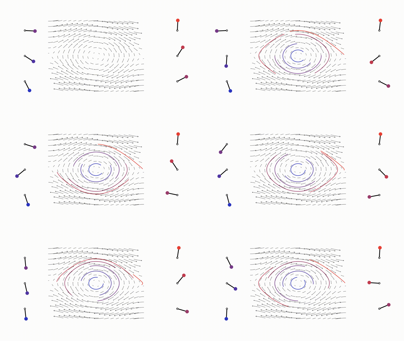
which hold because of the fact that the parameters $m,g,l$ are all positive. With this, we have that the real part of $\lambda(A(x_0))$ are both negative, and the real part of the second $\lambda(A(x_\pi))$ is positive. Therefore, the linearization about $A_0$ is stable, but for $A_\pi$, the system is unstable. This matches intuition; an upright pendulum falls over, whereas a freely swinging pendulum will eventually come to rest and the origin. By the Hartman-Grobman theorem, we know that the nonlinear system exhibits similar behavior around the fixed points. Below are depictions of the linearized system (blue) versus the nonlinear system (red) at various levels of magnification, decreasing from left to right.
 |
 |
 |
Lyapunov
What if, however, the linearization of the system was hyperbolic, as would be the case if $b$ were equal to zero. Lyapunov methods are more generalizable than linearization methods, and will be useful for constructing controllers in the subsequent sections. We will construct a candidate Lyapunov function from the Hamiltonian (total energy) of the system: \[ V(q) = H(\theta, \dot{\theta}) = T+V = \frac{1}{2}ml^2\dot{\theta}^2+mgl(1-\cos(\theta)). \] In order to determine the stability of the system, we differentiate $V(q(t))$ as in \begin{align} \dot{V}(q(t)) &= \frac{dV}{dq}f(q) = mgl\sin(\theta)\dot{\theta} + ml^2\dot{\theta}\ddot{\theta} \notag \\ &= mgl\sin(\theta)\dot{\theta}-ml^2\dot{\theta}(\frac{g}{l}\sin(\theta)+\frac{b}{ml^2}\dot{\theta}) \notag \\ &= -b\dot{\theta}^2 <0.\notag \end{align} Based on Lyapunov theory, because $V$ is a positive definite function, if $b=0$, then $\dot{V}\le 0$ implies stability of the system, which we know to be true. As before, if $b > 0$, $\dot{V}$ is negaitve definite, the system can be is determined to be locally asympotically stable about the origin $x_0$.
La Salle’s Theorem
Differential Geometry
The configuration manifold of the system is $\mathbb{S}^1$. Because $\mathbb{S}$ is isomorphic to $\mathbb{R}\backslash~$ where $~$ represents the equivalence class given by $\mathcal{R}={2\pi n}, n\in\mathbb{Z}$, the phase portrait should repeat iself every $2\pi$. Because $\mathbb{S}^1$ is a Lie group, the configuration manifold of this system is parallelizable, meaning $TQ\cong\mathbb{S}^1\times \mathbb{R}$. An interesting aside is that if we considered the $n$ pendulum (i.e. the connected pendulum with $n$ degrees of freedom), if $n$ were even, the configuration manifold would not be parallelizable by the Hairy Ball Theorem. In dynamical systems, the phase space of the system lies on tangent bundle, $TQ$.

Sources
https://physics.stackexchange.com/questions/343553/lagrangian-and-hamiltonian-formalism-for-damped-pendulum https://physics.stackexchange.com/questions/41034/what-are-the-reasons-for-leaving-the-dissipative-energy-term-out-of-the-hamilton https://ocw.mit.edu/courses/electrical-engineering-and-computer-science/6-241j-dynamic-systems-and-control-spring-2011/readings/MIT6_241JS11_chap13.pdf http://www.cfm.brown.edu/people/dobrush/am34/Mathematica/ch3/pendulum.html https://www.egr.msu.edu/~khalil/NonlinearSystems/Sample/Lect_9.pdf