The following discussion is meant to be a more illustrative exposition of the methodology employed in the paper: Multi-Rate Planning and Control of Uncertain Nonlinear Systems: Model Predictive Control and Control Lyapunov Functions, while answering some potential questions that may arise.
Table of Contents
Motivation
Before getting into the weeds, we will motivate the use of robust linear MPC, which will start with a discussion of linear MPC.
Linear MPC
First consider the deterministic linear conrol system with discrete time dynamics \[x_{k+1} = Ax_k + Bu_k\] with \(x\in \mathbb{R}^n\), \(u\in\mathbb{R}^m\), \(A\in\mathbb{R}^{n\times n}\), and \(B\in\mathbb{R}^{n\times m}\). The standard MPC program can be written as:
\begin{align}
u^* = \,\,\underset{u \in \mathbb{R}^m}{\text{argmin}} & \quad \sum_{k=0}^{N-1} x_k^\top Q x_k + u_k^\top R u_k + x_N^\top V x_N \notag\\ \notag
\mathrm{s.t.} \quad & \quad x_{k+1} = Ax_k + Bu_k \\ \notag
&\quad x_0 =x(0) \\ \notag
&\quad x_k \in \mathcal{X}\\ \notag
&\quad u_k \in \mathcal{U}\\ \notag
&\quad x_N \in \mathcal{X}_F, \nonumber
\end{align}
for \(Q\in\mathbb{R}^{n\times n}\), \(R\in\mathbb{R}^{m\times m}\) state and input weights, \(V\in\mathbb{R}^{n\times n}\) terminal cost, \(\mathcal{X}\subset \mathbb{R}^n\), \(\mathcal{U}\subset\mathbb{R}^m\), state and input constraints, and respectively, and \(\mathcal{X}_F\subset\mathbb{R}^n\) the terminal constraint set. For the sake of simplicity, we will start by assuming that the terminal constraint set is given by a point, i.e. \(x_e = \mathcal{X}_F\), which is a control invariant with control input \(u=0\).
Solving this optimization problem at time $t=0$ results in the optimal solutions:
\begin{align}
x^* &= \{x^*_{0|0},\ldots,x_e\}\notag \\
u^* &= \{u^*_{0|0},\ldots,u^*_{N-1|0}\}, \notag
\end{align}
where \(x_{k|t}\) represents the \(k^{th}\) state decision variable as planned at time index $t$, as depicted by:
 Consider the application of the open loop control action \(u^*_0\) at time step \(t=0\), resulting in the following system update:
 Of paramount importance with MPC is the notion of recursive feasibility, i.e. ensuring that if the program is feasible at instantiation, that it continues to be feasible at all times in the future. In the above diagram, it is clear to see that the following state and action pairs:
\begin{align}
x^* &= \{x^*_{1|0},\ldots,x_e, x_e\}\notag \\
Of paramount importance with MPC is the notion of recursive feasibility, i.e. ensuring that if the program is feasible at instantiation, that it continues to be feasible at all times in the future. In the above diagram, it is clear to see that the following state and action pairs:
\begin{align}
x^* &= \{x^*_{1|0},\ldots,x_e, x_e\}\notag \\
u^* &= \{u^*_{1|0},\ldots,u^*_{N-1|0}, 0\}, \notag
\end{align}
are feasible at time step \(t=1\) (again, assuming that \(x_e\), the terminal constraint set is a control invariant with control input \(u=0\). In general this idea can be extended to terminal constraints of arbitrary [polytopic, or more generally, convex] terminal constraints \(\mathcal{X}_F\)). To see this, consider the set \(\mathcal{X}_F\), a control invariant under the policy \(\pi:\mathbb{R}^n\to\mathbb{R}^m\). In the recursive feasability step, we can replace the state action pairs with:
\begin{align}
x^* &= \{x^*_{1|0},\ldots,x_{N|0}, Ax_{N|0} + B\pi(x_{N|0})\}\notag \\
u^* &= \{u^*_{1|0},\ldots,u^*_{N-1|0}, \pi(x_{N|0})\}, \notag
\end{align}
Robust Linear MPC
This is all fine and dandy, but now consider the uncertain system dynamics of \[x_{k+1} = Ax_k + Bu_k + w\] for \(w\in\mathcal{W}\subset\mathbb{R}^n\). In this setting, two things are lost:
- It may be that the system state exits the state constraint set
- We no longer have a guarantee of recursive feasibility
In order to remedy these issues, we have a few options. The first option is to plan policies over the disturbance set (more details can be found in this paper). It is not clear how to do this for general systems, but for linear systems with polytopic disturbance sets \(\mathcal{W}\), this can be achieved via an optimization program that is NP-hard to solve. Another option, which will naturally extend to nonlinear systems, is to use a feedback controller in tandem with MPC.
We start by defining a feedback policy \(K\in\mathbb{R}^{m\times n}\) which renders the closed loop system \(A_{\textrm{cl}} = A+BK\) stable. We can then generate a robust invariant \(\mathcal{E}\), i.e. a set such that for all elements \(x^-\in\mathcal{E}\), there exists an input \(u\) such that the point \(x^+ = Ax^-+Bu + w \in \mathcal{E}\) for all \(w\in\mathcal{W}\). The process of producing such a robust invariant for linear systems is depicted below, with more details in this paper.
 The notation \(\oplus\) is the Minkowski sum of two sets, i.e. given two sets \(A\) and \(B\), \(A\oplus B = \{a+b|a\in A, b\in B\}\), and \(\ominus\) is the Minkowski difference of two sets, i.e. if \(C=A\oplus B\) then \(A=C\ominus B\).
Although this set is not guaranteed to be polytopic, a polytopic outer approximation can readily be generated. Now, consider the following robust MPC program:
\begin{align}
(x,u)^* = \,\,\underset{x,u}{\text{argmin}} & \quad \sum_{k=0}^{N-1} x_k^\top Q x_k + u_k^\top R u_k + x_N^\top V x_N \notag\\ \notag
\mathrm{s.t.} \quad & \quad x_{k+1} = Ax_k + Bu_k \\ \notag
&\quad x_0 =x(0) \\ \notag
&\quad x_k \in \mathcal{X}\ominus \mathcal{E}\\ \notag
&\quad u_k \in \mathcal{U}\ominus K\mathcal{E}\\ \notag
&\quad x_N \in \mathcal{X}_F, \nonumber
\end{align}
where it must be verified that \(\mathcal{X}\ominus \mathcal{E}\) and \(U\ominus K\mathcal{E}\) are not empty, and that \(\mathcal{X}_F\subset\mathcal{X}\ominus\mathcal{E}\). From the solutions \((x,u)^*\), the control input to the system can be constructed as: \[\pi(x) = K(x-x^*_{0|0})+u^*_{0|0}.\]
This formulation grants us a number of benefits. First, it resolves the two aforementioned challenges, i.e. the states (and inputs) will remain in the constraint sets, and recursive feasibility can be guaranteed. To see this, consider the optimal sequence of states at time step \(t=0\):
The notation \(\oplus\) is the Minkowski sum of two sets, i.e. given two sets \(A\) and \(B\), \(A\oplus B = \{a+b|a\in A, b\in B\}\), and \(\ominus\) is the Minkowski difference of two sets, i.e. if \(C=A\oplus B\) then \(A=C\ominus B\).
Although this set is not guaranteed to be polytopic, a polytopic outer approximation can readily be generated. Now, consider the following robust MPC program:
\begin{align}
(x,u)^* = \,\,\underset{x,u}{\text{argmin}} & \quad \sum_{k=0}^{N-1} x_k^\top Q x_k + u_k^\top R u_k + x_N^\top V x_N \notag\\ \notag
\mathrm{s.t.} \quad & \quad x_{k+1} = Ax_k + Bu_k \\ \notag
&\quad x_0 =x(0) \\ \notag
&\quad x_k \in \mathcal{X}\ominus \mathcal{E}\\ \notag
&\quad u_k \in \mathcal{U}\ominus K\mathcal{E}\\ \notag
&\quad x_N \in \mathcal{X}_F, \nonumber
\end{align}
where it must be verified that \(\mathcal{X}\ominus \mathcal{E}\) and \(U\ominus K\mathcal{E}\) are not empty, and that \(\mathcal{X}_F\subset\mathcal{X}\ominus\mathcal{E}\). From the solutions \((x,u)^*\), the control input to the system can be constructed as: \[\pi(x) = K(x-x^*_{0|0})+u^*_{0|0}.\]
This formulation grants us a number of benefits. First, it resolves the two aforementioned challenges, i.e. the states (and inputs) will remain in the constraint sets, and recursive feasibility can be guaranteed. To see this, consider the optimal sequence of states at time step \(t=0\):
 Then, once the policy is applied, we can simply use the same sequence of states and inputs that were used in the previous section (depending on if the terminal set is an unforced equilibrium point, or more generally a control invariant), which are feasible at the next time step:
 Additionally, this formulation does all of this while avoiding having to solve an NP-hard problem.
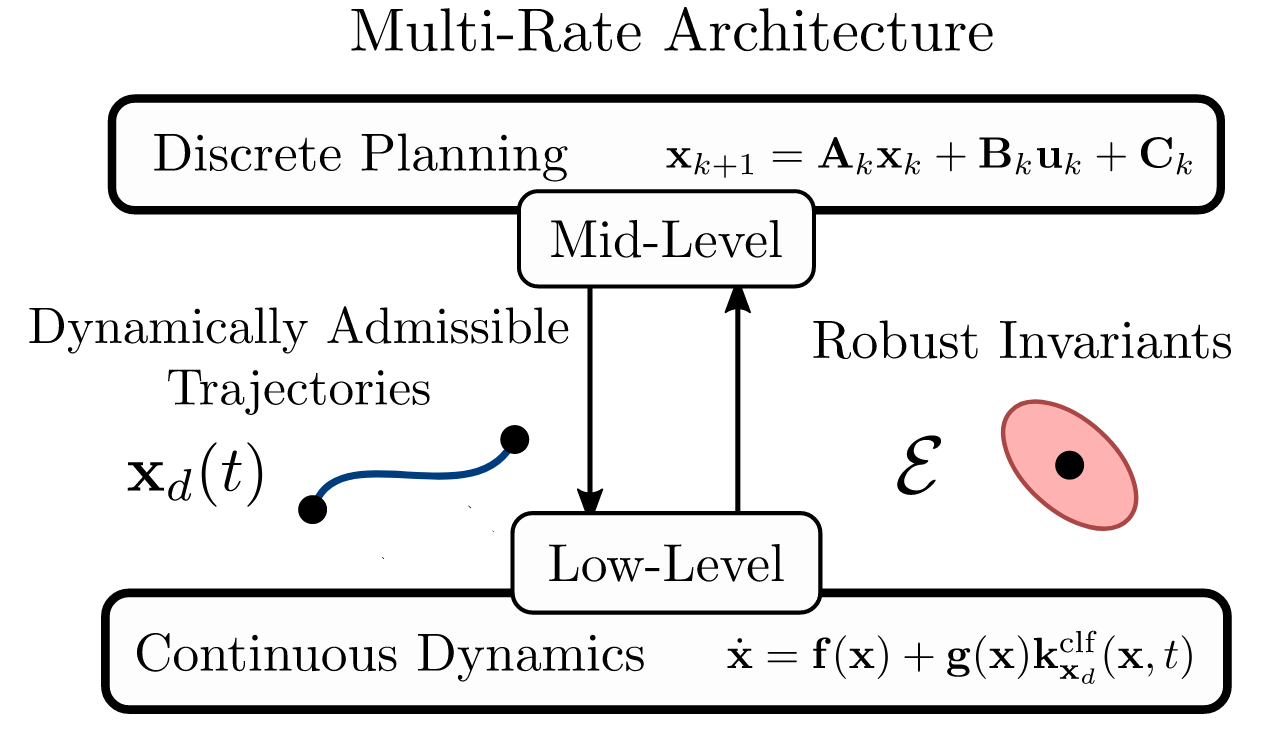
This paradigm of separating the feedback to a “low-level” controller, allowing the MPC program to plan over the disturbance free system is the same idea as employed in my most recent paper), which extends this concept to nonlinear systems: