Table of Contents
The Goal of Control
Given a physical system, it seems natural to wish for it to exhibit desired behavior. For example, if I have a robot, I want it to do \({something}\). The goal of control theory is to certifiably drive dynamical systems \(\dot x = f(x)\) to desired states \(x^*\). Without (much) loss of generality, we can describe achieving the desired behavior as minimizing \(\|x(t)-x^*\|\) for some desired state \(x^*\). Therefore, of paramount importance is the notion of stability, which captures the ability of the system to decrease, or at the very least bound, the error between the actual system state and the desired state. These notions are formalized as follows:
Stability:
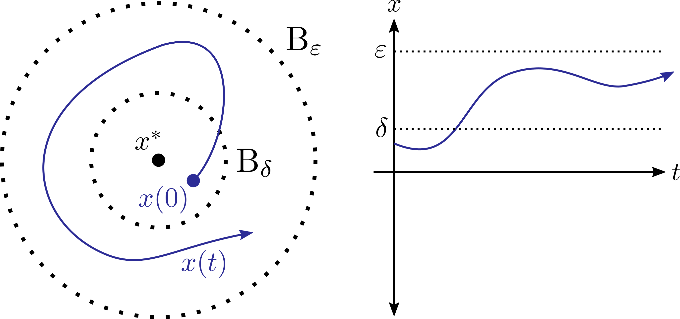
A system is stable if, for all \(\varepsilon>0\), there exists a \(\delta>0\) such that: \[\|x(0)-x^*\| < \delta \implies \|x(t)-x^* \| < \varepsilon,~~~~ \forall t\ge 0.\]
Asymptotic Stability:
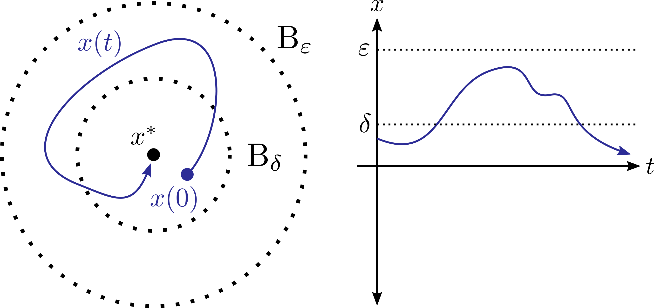
A system is asymptotically stable if it is stable, and additionally: \[\lim_{t\to\infty}\|x(t)-x^*\| = 0 \]
Exponential Stability:
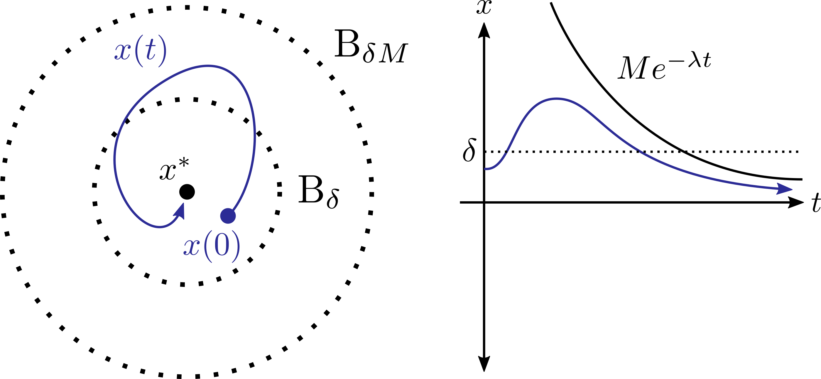
A system is exponentially stable if there exists \(M,\lambda,\delta>0\) such that: \[ \|x(0)-x^*\| \le \delta \implies \|x(t) - x^*\| \le Me^{-\lambda t}\|x(0)-x^*\|. \]
Thus far, discussing the stability of the system relies on being able to describe \(x(t)\), which is largely impossible to compute for nonlinear systems (even for a system as simple as the pendulum). Luckily, Lyapunov’s method of stability allows us to reason about the stability of systems without needing to explicitly solve for their solution.
Lyapunov’s Method
Instead of thinking about what the system will do as time progresses, we can instead think about how a property of the system evolves over time. For example, if I know that the energy of a mechanical system is (strictly) decreasing over time, I don’t have to know exactly what it will do to conclude that it will eventually come to a rest (i.e. will be asymptotically stable). Lyapunov’s method does exactly this, and Lyapunov functions can in some ways be though of as a generalization of energy functions.
Lyapunov’s Theorem
Let \(V:\mathbb{R}^n\to\mathbb{R}\) be a continuously differentiable function satisfying \(V(0) = 0\). If \(V\) additionally satisfies:
- \(V(x) \succ 0\) (positive definite),
- \(\dot V(x) \le 0\),
then (the equilibrium) \(x^*\) is stable.
Proof
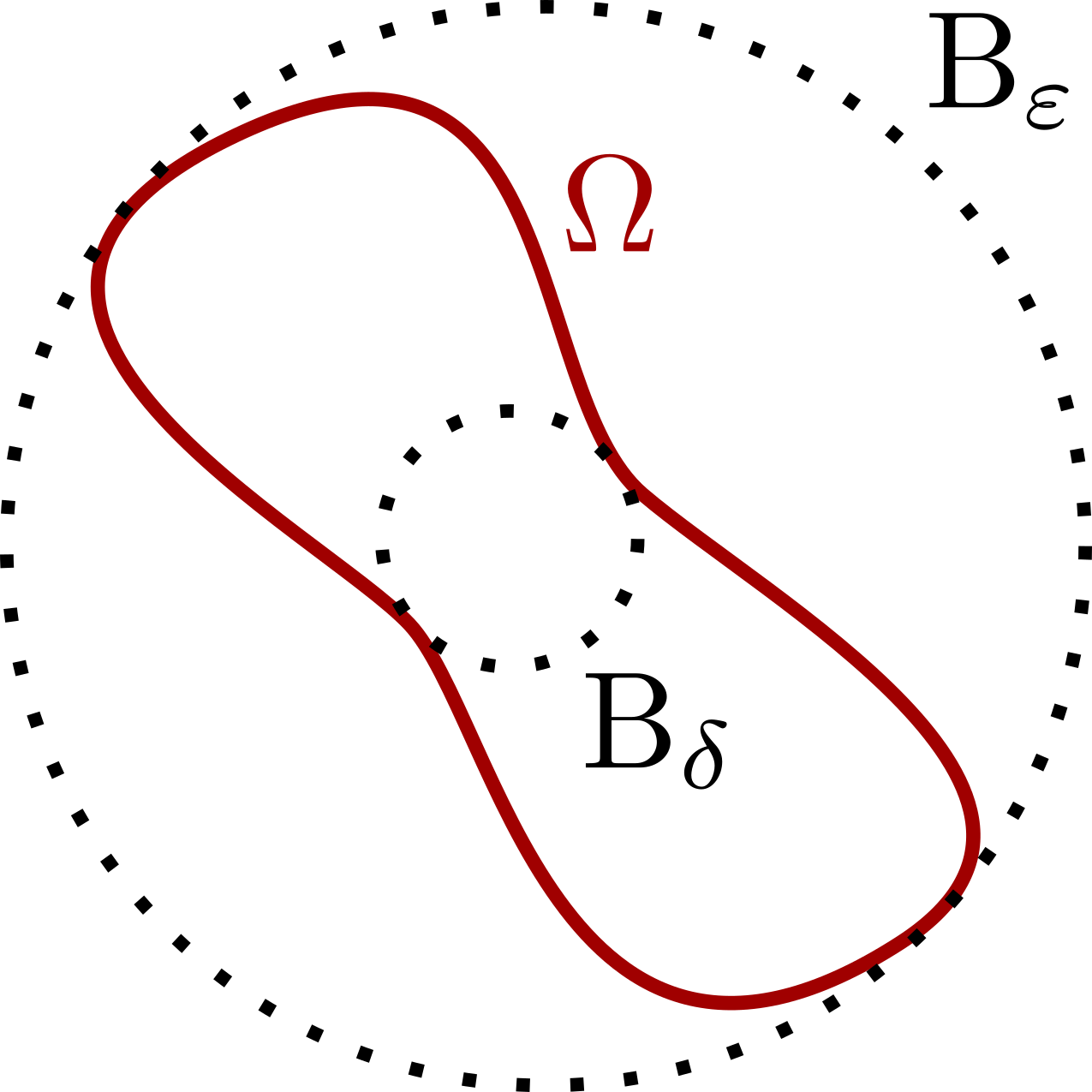 Given an \(\varepsilon>0\), consider the Lyapunov sublevel set \(\Omega=\{x\in\mathbb{R}^n : V(x) \le c\}\) for some \(c\) such that \(\Omega \subset B_\varepsilon(0)\).
Such a construction is possible via the combined continuity and positive definiteness of \(V.\) Next, observe the following:
\[
V(x(t)) = V(x(0)) + \int_0^t \underbrace{\dot{V}(x(t))}_{\le 0} dt \le V(x(0)) \le c.
\]
Therefore, for initial conditions starting in \(\Omega\), they will remain in \(\Omega\) for all time, i.e. the set \(\Omega\) is forward invariant. With this, define \(\delta > 0\) such that \(B_\delta(0) \subset \Omega\), leading to:
\[
x(0) \in B_\delta(0) \implies x(0) \in \Omega \implies x(t) \in \Omega \implies x(t) \in B_\varepsilon(0),~~~~\forall t\ge 0,
\]
or equivalently:
\[
\|x(0)\| < \delta \implies \|x(t)\|< \varepsilon,
\]
i.e. the system is stable. \(\tag*{$\Box$}\)
Given an \(\varepsilon>0\), consider the Lyapunov sublevel set \(\Omega=\{x\in\mathbb{R}^n : V(x) \le c\}\) for some \(c\) such that \(\Omega \subset B_\varepsilon(0)\).
Such a construction is possible via the combined continuity and positive definiteness of \(V.\) Next, observe the following:
\[
V(x(t)) = V(x(0)) + \int_0^t \underbrace{\dot{V}(x(t))}_{\le 0} dt \le V(x(0)) \le c.
\]
Therefore, for initial conditions starting in \(\Omega\), they will remain in \(\Omega\) for all time, i.e. the set \(\Omega\) is forward invariant. With this, define \(\delta > 0\) such that \(B_\delta(0) \subset \Omega\), leading to:
\[
x(0) \in B_\delta(0) \implies x(0) \in \Omega \implies x(t) \in \Omega \implies x(t) \in B_\varepsilon(0),~~~~\forall t\ge 0,
\]
or equivalently:
\[
\|x(0)\| < \delta \implies \|x(t)\|< \varepsilon,
\]
i.e. the system is stable. \(\tag*{$\Box$}\)
Finally, the assumptions of the theorem can be strengthened to show other forms of stability. Namely, asymptotic stability can be certified if \(\dot V \prec 0\) (is negative definite), and exponential stability if \(\dot V \le -\gamma V\) for some \(\gamma > 0\).
Some Further Intuition
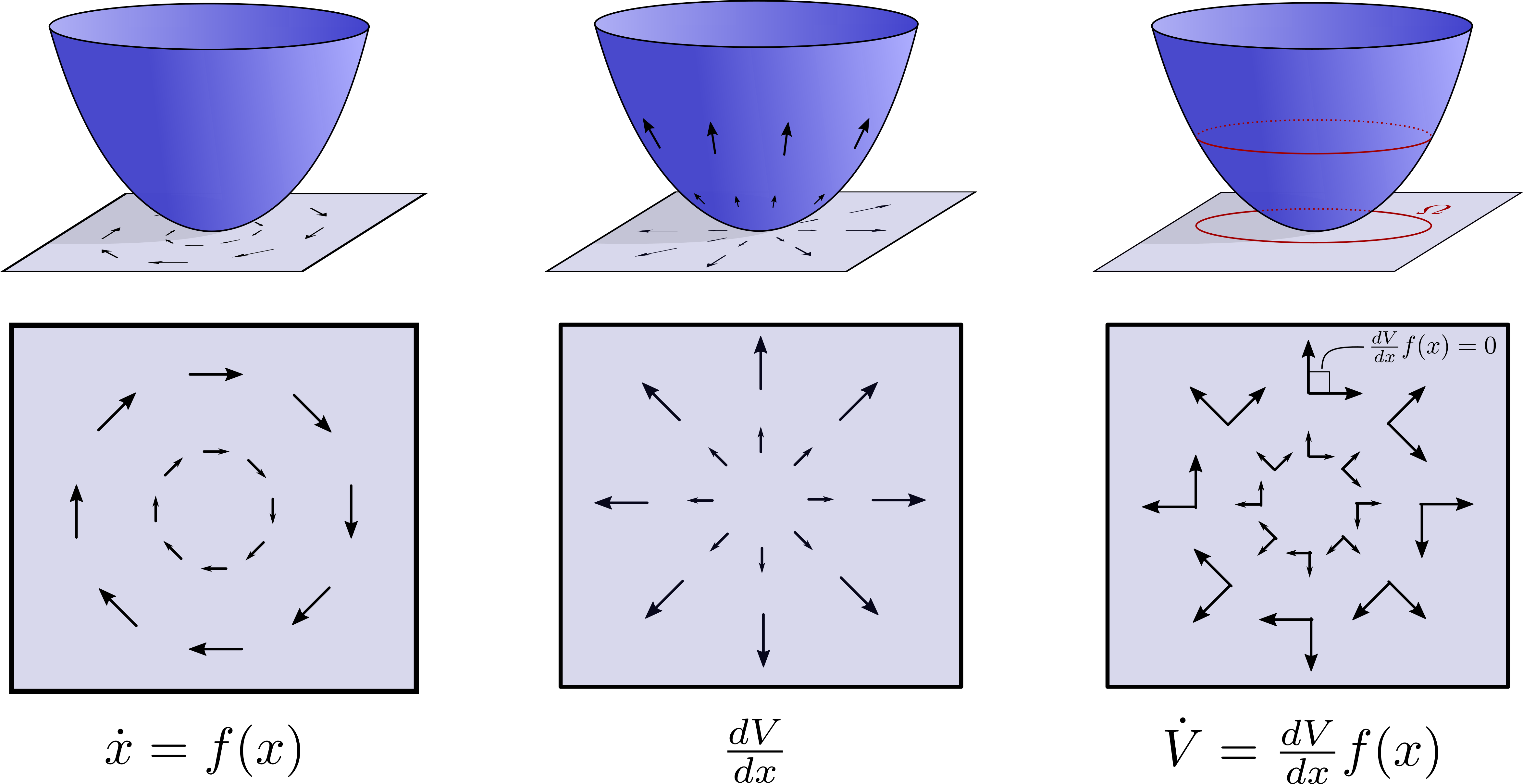
Although the proof is quite simple, it is useful to think deeper about the operations going on under the hood in order to gain some better intuition. First, observe that the time derivative of \(V\) is given by: \[ \dot V(x) = \frac{dV}{dx} \dot x = \frac{dV}{dx}f(x), \] due to the chain rule. This can alternatively be though of as an inner product between vector fields: the vector field generated by taking the gradient of the scalar function \(V\), which points in the direction of steepest ascent, and the vector field \(f\) associated with the dynamics of the system. A dot product measures the extent to which to vectors “align”, so measuring \(\dot V\) is really assessing the extent to which the dynamics will increase the value of the Lyapunov function \(V\). If this derivative is zero, then the vectors \(\frac{dV}{dx}\) and \(f\) are orthogonal. Therefore, the flow of the system will maintain the value of the Lyapunov function – the system will stay on level sets. On the other hand, if the inner product is negative, then some component of the dynamics are pointing in a direction that will decrease the Lyapunov function, and if this happens at all points in time then the system must asymptotically approach the origin. These ideas are captured via the following image: