Table of Contents
Theorem
Every continuous function $f:D^n\to D^n$ has a fixed point, i.e. a point $x\in D^n$ such that $f(x) = x$.
Preface to the Proof
There are many ways to prove the above statement, but an especially elegant method utilizes the functorality of homology. In order to see this, we need to build up some preliminaries. For the following discussion, we will use $S^2$ as the motivating example, but the presented ideas can be extended to a wide variety of topological spaces.
Simplicial Homology
What is a simplex?
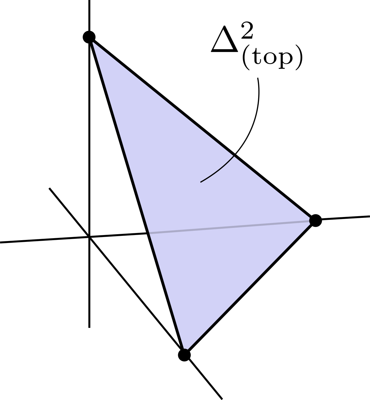
A topological n-simplex $\Delta^n_{\textrm{(top)}}$ is defined as \[\Delta^n_{\textrm{(top)}} = \{t=(t_0,\ldots,t_n)\in\mathbb{R}^{n+1}:t_i \ge 0,\sum t_i = 1\}.\] For example, the topological two simplex is:
Delta Complexes
$\Delta$-complexes ($\Delta$-cxs), like simplicial and a CW-complexes, are a collection of maps $\sigma:\Delta^n\to X$ which take simplices and glue them together in specific ways to form topological spaces. Specifically, this process is done inductively, where at each step you add a new simplex by gluing its boundary to the existing complex via a map $g$. For $\Delta$-complexes, simply stated, the map $g$ must glue together faces in the canonical way (linearly, and preserving ordering of the vertices).
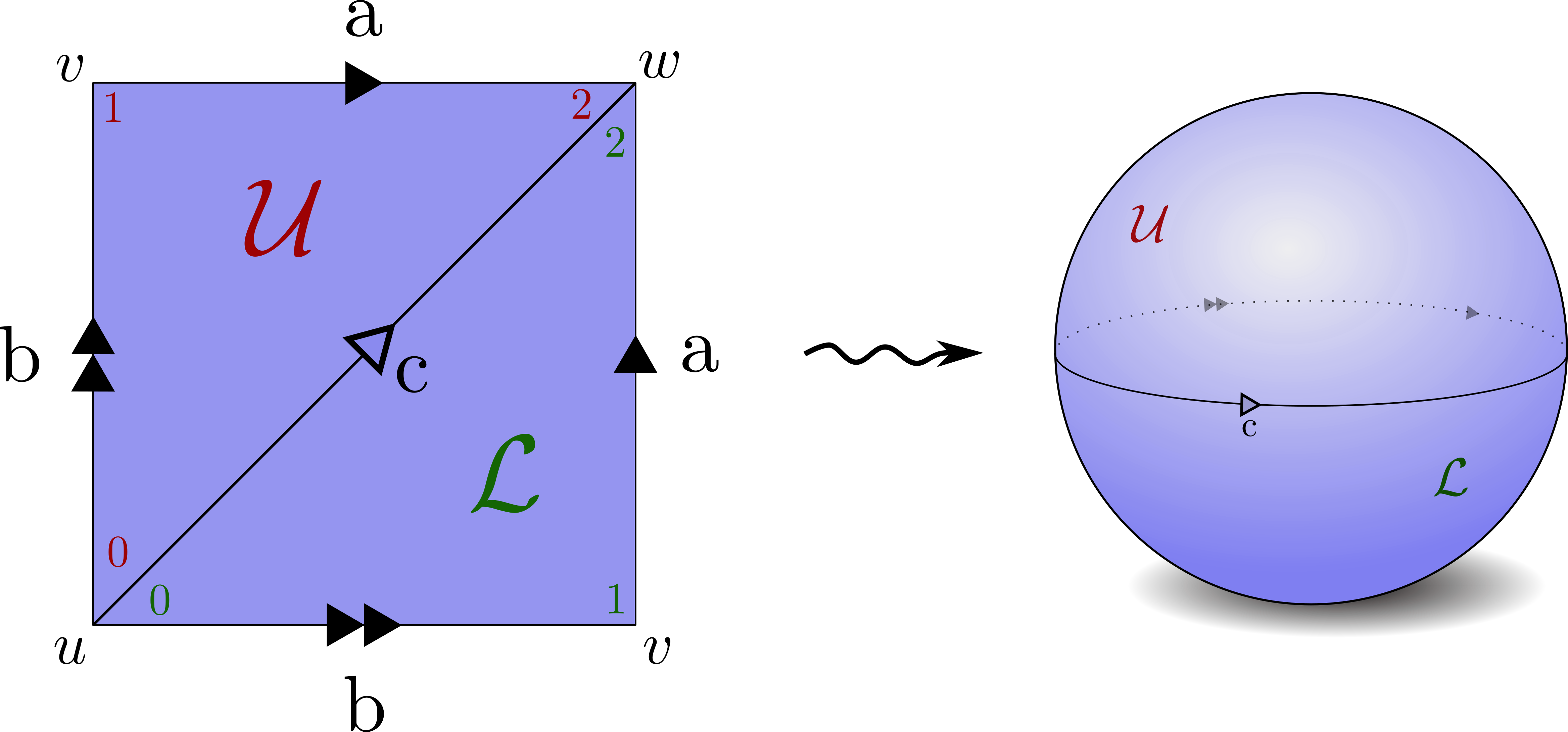
We can create a $\Delta$-cx structure on $S^2$ in the following way:
The relationship between simplices of different dimensions on the same topological space can be described via chain complexes.
What is a Chain Complex?
A chain complex (of Abelian groups) is a sequence of Abelian groups and group homomorphims: \[ C_\bullet = \left( \ldots \xrightarrow{\partial_{n+1}} C_n \xrightarrow{\partial_n} C_{n-1} \xrightarrow{\partial_{n-1}} C_{n-2} \ldots \right) \] such that $\partial_n\circ\partial_{n+1} = 0$. We can derive chain complexes from $\Delta$-cxs in the following way: Let $C_n$ for $n\in\mathbb{N}$ be the free Abelian group generated by $n$-simplices in $X$, $\sigma_n$. In other words we simply treat $\sigma$ as a symbol, and generate a free group by applying the usual rules of addition and subtraction.
For every element $i\in\{0,\ldots,n\}$, we can define the $i$-th face $\delta_i^n\subset\Delta^n$ to be \[ \delta_i^n = \{t\in\Delta^n:t_i = 0\} \]
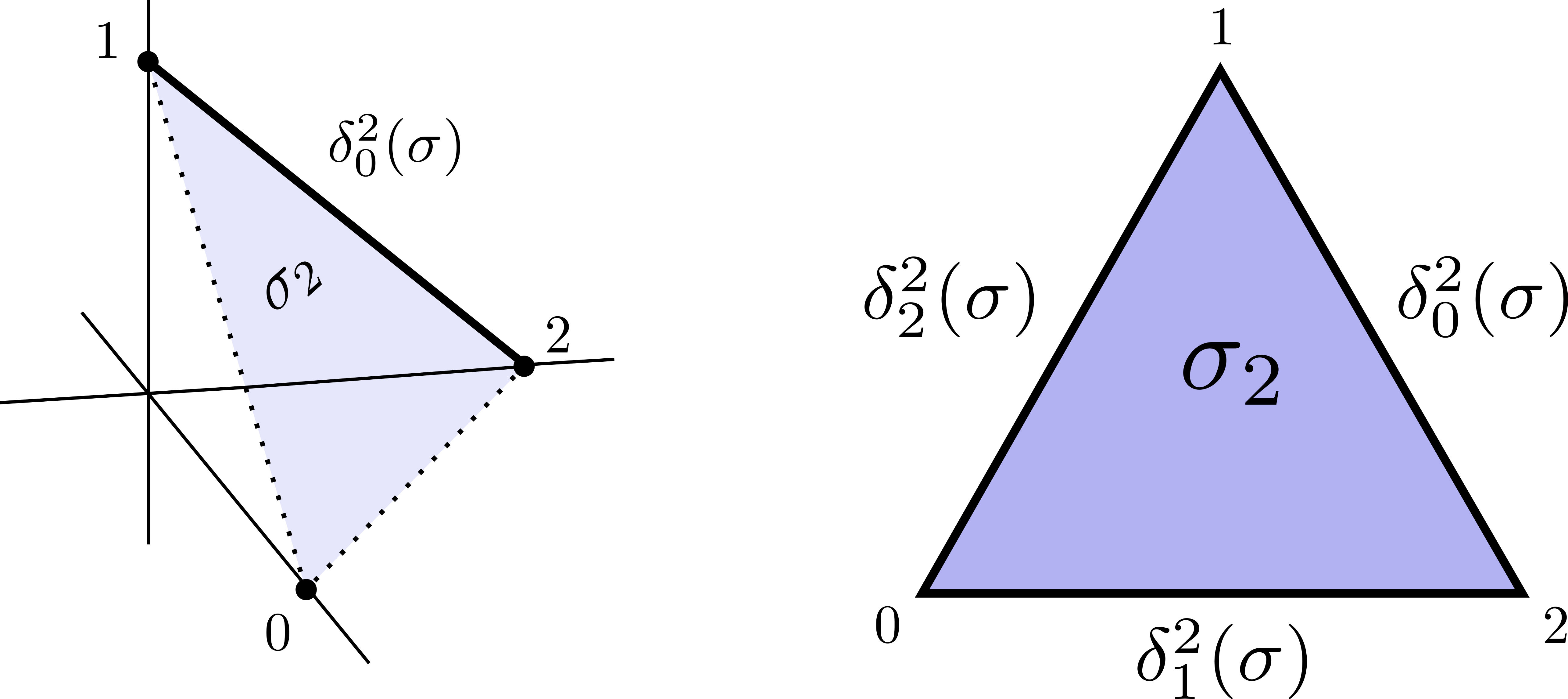
The boundary of $\sigma_n$ is defined as the formal sum of the $(n-1)$ simplices that are the restriction of $\sigma$ to the faces of $\Delta^n$, with alternating sign. In other words:
\[
\partial \sigma_n = \sum_{i=0}^n(-1)^i\delta_i^n
\]
Each simplex is oriented, and we state that a simplex is equal to the negative of the simplex with the opposite orientation. In the example of the sphere, we have the following boundary maps:
\[
\begin{align}
\partial_1 \sigma_a &= w-v \notag \\
\partial_1 \sigma_b &= v-u \notag \\
\partial_1 \sigma_c &= w-u \notag \\
\partial_2 \sigma_U &= a-c+b \notag \\
\partial_2 \sigma_L &= a-c+b \notag \\
\end{align}
\]
Furthermore, we can verify that $\partial \circ \partial = 0$, for example
\[
\partial(\partial \sigma_L) = \partial(a-c+b) = (w-v)-(w-u)+(v-u) = 0
\]
The boundary map can also be viewed as a map $\partial:C_n(X)\to C_{n-1}(X)$, and from these maps we can create a chain complex. So, for our running example, we have
\[
\begin{align}
C_\bullet^\Delta(S^2) &= \left( C_3(X) \xrightarrow{\partial_3} C_2(X) \xrightarrow{\partial_2} C_1(X) \xrightarrow{\partial_1} C_0(X) \xrightarrow{\partial_0} 0\right) \notag \\
&= \left( 0 \xrightarrow{\partial_3} \mathbb{Z}\{\mathcal{U},\mathcal{L}\} \xrightarrow{\partial_2} \mathbb{Z}\{\textrm{a,b,c}\} \xrightarrow{\partial_1} \mathbb{Z}\{u,v,w\} \xrightarrow{\partial_0} 0\right) \notag
\end{align}
\]
What is Homology?
In order to define homology, we must first understand cycles and boundaries. An $n$-chain $C_n(X)$ is said to be an $n-cycle$, denoted as $Z_n$, if its boundary is zero: \[ \sigma \in Z_n \implies \partial \sigma = 0. \] An $n$-cycle is an $n-boundary$, denoted as $B_n$, if it is the boundary of an $(n+1)$ chain of X: \[ \sigma \in B_n \implies \sigma \in Z_n,~\text{and}~\exists \sigma’\in C_{n+1}~\text{s.t.}~\partial_{n+1} \sigma’ = \sigma. \] So, given the boundary maps $\partial_n$, what are the groups $Z_n$ and $B_n$? Well, $B_n$ is simply the image of $\partial_{n+1}$, which takes $n+1$ simplices and extracts their boundaries. On the other hand, $Z_n$ is the kernel of $\partial_{n}$, because the kernel of the map tells us which elements have zero boundary. As every element of $B_n$ must be an element of $Z_n$, we can form a quotient space – this quotient space is the homology! Specifically, \[ H^\Delta_n(X) := H_n(C^\Delta_\bullet(X)) = \frac{Z_n}{B_n} \] Informally, the $n^{th}$ homology measures $n$-dimensional holes of our space $X$, which are exactly the cycles ($n$ dimensional “loops”) that are not the boundary of anything in one dimension higher.
Let’s continue with our running example and perform some calculations on $S^2$:
\[
\begin{align}
ker(\partial_2) &= \{x\cdot \mathcal{U} + y\cdot \mathcal{L} : x,y\in\mathbb{Z}, \partial_2 (x\cdot \mathcal{U} + y\cdot \mathcal{L}) = 0\} \notag \\
&= \{x\cdot \mathcal{U} + y\cdot \mathcal{L} : x,y\in\mathbb{Z}, x \cdot \partial_2 \mathcal{U} + y\cdot \partial_2\mathcal{L} = 0\} \notag \\
&= \{x\cdot \mathcal{U} + y\cdot \mathcal{L} : x,y\in\mathbb{Z}, x \cdot (a-c+b) + y\cdot (a-c+b) = 0\} \notag \\
&= \{x\cdot \mathcal{U} + y\cdot \mathcal{L} : x,y\in\mathbb{Z}, (x + y) \cdot (a-c+b) = 0 = 0\} \notag \\
&= \{x\cdot \mathcal{U} + y\cdot \mathcal{L} : x,y\in\mathbb{Z}, x = -y \} \notag \\
&= \mathbb{Z}\{\mathcal{U} - \mathcal{L}\} \notag
\end{align}
\]
\[
\begin{align}
ker(\partial_1) &= \{x\cdot a + y\cdot b +z\cdot c : x,y,z\in\mathbb{Z}, \partial_1 (x\cdot a + y\cdot b + z\cdot c) = 0\} \notag \\
&= \{x\cdot a + y\cdot b +z\cdot c : x,y,z\in\mathbb{Z}, x \cdot (w-v) + y \cdot (v-u) + z\cdot (w-u) = 0 \} \notag \\
&= \{x\cdot a + y\cdot b +z\cdot c : x,y,z\in\mathbb{Z}, (x+z) = (x+y) = (y-z) = 0\} \notag \\
&= \mathbb{Z}\{c-a+b\} \notag \\
\end{align}
\]
\[
\begin{align}
ker(\partial_0) &= \mathbb{Z}\{u,v,w\} \notag
\end{align}
\]
\[
\begin{align}
im(\partial_3) &= 0 \notag
\end{align}
\]
\[
\begin{align}
im(\partial_2) &= \mathbb{Z}\{c-b+a\} \notag
\end{align}
\]
\[
\begin{align}
im(\partial_1) &= \mathbb{Z}\{w-v, u-v, w-u\} \notag
\end{align}
\]
Performing the quotient calculations yields the following homology groups for $S^2$:
\[
\begin{align}
H^\Delta_2(S^2) &= \frac{Z_2}{B_2} = \frac{ker(\partial_2)}{im(\partial_3)} = \frac{\mathbb{Z}\{\mathcal{U} - \mathcal{L}\}}{0} = \mathbb{Z} \notag \\
H^\Delta_1(S^2) &= \frac{Z_1}{B_1} = \frac{ker(\partial_1)}{im(\partial_2)} = \frac{\mathbb{Z}\{c-a+b\}}{\mathbb{Z}\{c-a+b\}} = 0 \notag \\
H^\Delta_0(S^2) &= \frac{Z_0}{B_0} = \frac{ker(\partial_0)}{im(\partial_1)} = \frac{\mathbb{Z}\{u,v,w\}}{\mathbb{Z}\{w-v, u-v, w-u\}} = \mathbb{Z} \notag \\
\end{align}
\]
The above triangulations can be created for $S^n$ for $n\in\mathbb{N}$, but this would be quite an annoying calculation to perform. This annoyance calls for a slight digression into cellular homology.
Cellular Homology
Although simplices and simplicial homology are very algorithmic to compute, they can be exceedingly cumbersome as dimensionality grows. As such, there exits an alternative – cellular homology – which is less rigid and often more useful, and relies on CW-complexes instead of $\Delta$-complexes. These homologies are not only isomorphic, but also lead to the same chain complexes; therefore, the computations related to homology must agree.
The above computation can also be performed (more directly) for the $n$-sphere with CW complexes by noting that the $S^n$ has cell structure in only the zeroth and $n^{th}$ levels. With this observation we can immediately conclude that:
\[
H_k(S^n) =
\begin{cases}
\mathbb{Z},&k=0,n \\
0,& \text{o.w.}
\end{cases}
\]
Singular Homology
In fact, there is an even more general version of homology (often too general to be used in direct computation), called singular homology. Importantly, singular homology is a functor \[ H_n: \textbf{Top}\to\textbf{Ab} \] from the category $\textbf{Top}$, with objects topological spaces and morphisms continuous maps, and the category $\textbf{Ab}$ with objects Abelian groups and morphisms group homomorphisms. This can be seen by observing that singular $n$-chains are also functors $C_n:\textbf{Top}\to \textbf{Ab}$ (continuous functions between topological spaces induces group homomorphisms on $n$-chains), and the boundary map commutes with continuous maps. The functorality of singular homology, as well as its isomrphisms with other homology types is key for a number of applications of homology.
Reduced homology
Reduced homology, $\tilde H_i$, is simply a bookkeeping tool to remove the extra copy of $\mathbb{Z}$ in the lowest dimension. In other words
\[
\begin{align}
H_k &\cong \tilde H_k,~~~k\ge 1 \notag \\
H_0 &\cong \tilde H_0 \oplus \mathbb{Z}. \notag
\end{align}
\]
Back to the Proof
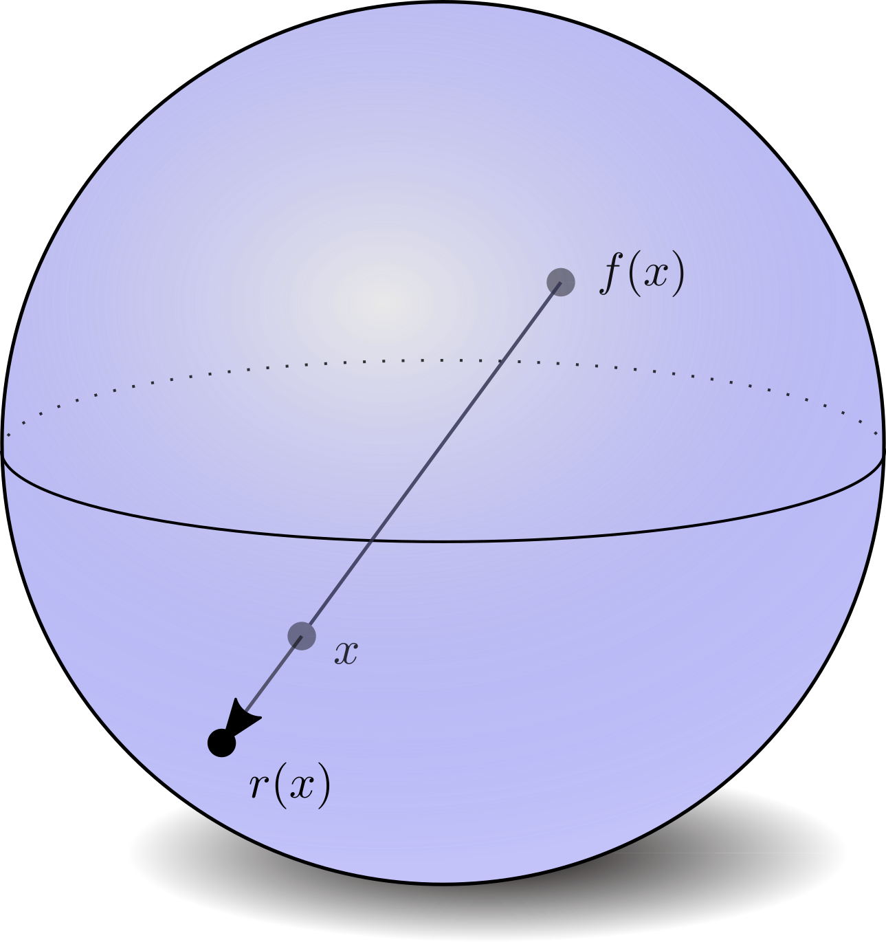
Let’s repeat the claim: Every continuous function $f:D^n\to D^n$ has a fixed point, i.e. a point $x\in D^n$ such that $f(x) = x$. We begin by assuming for the sake of contradiction that such a continuous function $f$ exists with no fixed points. This would guarantee that the points $x,f(x) \in D^n$ are distinct. As such, it would be possible to construct a retraction $r:D^n \to S^{n-1}$ from the disk to its boundary $\partial D^n = S^{n-1}$ via a ray from $f(x)$ passing through the $x$ to $S^{n-1}$, as depicted below:
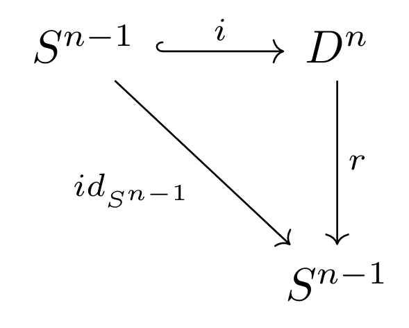
Defining the inclusion map as $i:S^{n-1}\to D^n$, the retraction $r$ would be a continuous function such that $r\circ i=id_{S^{n-1}}$. This can be depicted diagrammatically as:
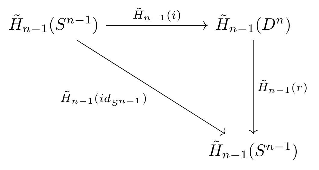
Note that this commutative diagram exists in the category $\textbf{Top}$; as such we can apply the homology functor! Applying the (reduced) singular homology functor, we have:
As singular homology is isomorphic to both cellular and simplicial homology, we can substitute the values calculated above, and therefore can replace the above diagram with the following:
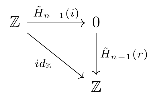
where $\tilde H_{n-1}(id_{S^{n-1}}) = id_{\tilde H_{n-1}(S^{n-1})} = id_{\mathbb{Z}}$ due to the functorality of homology (functors preserve identity maps). The result becomes clear: for all values of $n>0$, the identity map on the integers cannot factor through zero. Namely, no function exists mapping zero to the entirety of the integers, as functions map inputs to individual outputs, and there is only one input to map from. (The case when $n=0$ is trivial, as $D^0=pt$, which must be a fixed point). As such, we can conclude that no such function $f$ can exist for any dimension $n$. How beautiful!
Resources
Hatcher
Singular Homology Wiki
Chain Complex Wiki
nLab Reduced Homology
Formal Sum of Simplices StackExchange
Duality
An Introduction to Homology
Algebraic Topology Notes
Delta complex vs CW complex vs Simplicial complex StackExchange
Complexes and Associated Homologies StackExchange
Brouwer’s Fixed Point Theorem (n=2)